Glass Catalog Spreadsheets and Python
Optical glass manufacturers have settled on Excel spreadsheets as a means of documenting the technical details of their glass products. The formats are broadly similar but different in the details.
A major goal of the OpticalGlass package is to make the data in these vendor spreadsheets accessible to the Python user. OpticalGlass uses the pandas package to import and save the glass catalog in a DataFrame. These Excel spreadsheet catalogs are added to the ‘xls’ library, og_glass_libs[‘xls’].
Common data categories across all vendors include:
‘refractive indices’
‘dispersion coefficients’
‘internal transmission mm, 10’
‘chemical properties’
‘thermal properties’
‘mechanical properties’
These queries on the glass catalog dataframe return pandas Series with the data and (typically) the wavelengths used for sampling. These can be easily accessed as numpy arrays and can be plotted using matplotlib style capabilities.
The catalogs also contain single items of interest. The 2 that are supported across all catalogs currently include:
‘abbe number’
‘specific gravity’
A higher level interface is available as a set of catalog-specific subclasses of GlassPandas.
%matplotlib inline
Import glass and catalog factory functions.
import numpy as np
import matplotlib.pyplot as plt

from opticalglass.glassfactory import create_glass, og_glass_libs
catalog = 'Hoya'
gname = 'FCD1'
gname1 = 'E-F2'
gname2 = 'MC-TAF1'
Importing a catalog spreadsheet
The initialization of the global variable og_glass_libs reads the Excel spreadsheet into a DataFrame. A requirement for the import process is that the spreadsheet data be copied untouched into the catalog DataFrame. Only the spreadsheet row and column headers are changed in creating the catalog DataFrame.
The GlassCatalogPandas.df attribute has the glass catalog DataFrame.
hoya_xls = og_glass_libs['xls']['Hoya']
hoya_df = hoya_xls.df
Listing a catalog’s data categories
The column categories can be listed using the get_level_values() method and eliminating duplicates. Categories defined by OpticalGlass are all lower case.
hoya_df.columns.get_level_values(0).drop_duplicates()
Index([                                                                  'Code',
                                                             'refractive index',
                                                                  'abbe number',
                                                           'refractive indices',
                                                                        'blank',
                                                      'dispersion coefficients',
                                                          'Partial Dispersions',
                                                    'Partial Dispersion Ratio ',
                                    'Deviation of Relative Partial Dispersions',
                                                          'chemical properties',
                                                           'thermal properties',
                                                        'mechanical properties',
                                  'Temperature Coefficient of Refractive Index',
                                                                            nan,
          'Temperature Coefficient of Refractive Index  nh  404.66   (×10-6/℃)',
          'Temperature Coefficient of Refractive Index  ng  435.84   (×10-6/℃)',
          'Temperature Coefficient of Refractive Index  nF' 479.99   (×10-6/℃)',
          'Temperature Coefficient of Refractive Index  nF  486.13   (×10-6/℃)',
          'Temperature Coefficient of Refractive Index  ne  546.07   (×10-6/℃)',
          'Temperature Coefficient of Refractive Index  nd  587.56   (×10-6/℃)',
       'Temperature Coefficient of Refractive Index  nHe-Ne  632.8   (×10-6/℃)',
          'Temperature Coefficient of Refractive Index  nC' 643.85   (×10-6/℃)',
          'Temperature Coefficient of Refractive Index  nC  656.27   (×10-6/℃)',
           'Temperature Coefficient of Refractive Index  nr 706.52   (×10-6/℃)',
            'Temperature Coefficient of Abbe number  dνd/dT 587.56   (×10-3/℃)',
            'Temperature Coefficient of Abbe number  dνe/dT 546.07   (×10-3/℃)',
                             'Refractive index change to the cooling velocity ',
                                                  'Stress Optical Coefficient ',
                                                             'specific gravity',
                                                      'Spectral Transmittance ',
                                                  'internal transmission mm, 2',
                                                  'internal transmission mm, 5',
                                                 'internal transmission mm, 10',
                                                  'Glass Cross Reference Index',
                                                                      'Remarks',
                                                                       'Update'],
      dtype='object', name='category')
The glass_data() method returns a Series of the catalog data for the specified glass name.
fcd1_pd = hoya_xls.glass_data('FCD1')
The standard data categories can then be used to access the specific glass’s data.
The 'dispersion coefficients' category give the glass’s dispersion polynomial coefficients.
fcd1_pd['dispersion coefficients']
data item
A0       2.218113
A0pow           0
A1      -5.799427
A1pow          -3
A2       8.347068
A2pow          -3
A3       6.504652
A3pow          -5
A4       8.514219
A4pow          -6
A5      -5.885227
A5pow          -7
Name: FCD1, dtype: object
The 'refractive indices' category gives the measured refractive indices at measurement wavelengths.
fcd1_pd['refractive indices']
data item
1529.6     1.48598
1128.64    1.48907
t          1.49008
s          1.49182
A'           1.493
r          1.49408
C          1.49514
C'         1.49543
He-Ne      1.49571
D          1.49694
d            1.497
e          1.49845
F          1.50123
F'         1.50157
g          1.50451
h          1.50721
i          1.51175
Name: FCD1, dtype: object
The refractive index at a particular spectral line can be obtained with an additional level of indexing.
fcd1_pd['refractive indices']["F'"]
np.float64(1.50157)
Data can be returned in numpy arrays using the pandas conversion function to_numpy()
indices = fcd1_pd['refractive indices'].to_numpy(dtype=float); indices
array([1.48598, 1.48907, 1.49008, 1.49182, 1.493  , 1.49408, 1.49514,
       1.49543, 1.49571, 1.49694, 1.497  , 1.49845, 1.50123, 1.50157,
       1.50451, 1.50721, 1.51175])
Transmission data for 10mm thick samples is available.
fcd1_pd['internal transmission mm, 10']
data item
2500      0.999
2400.0    0.999
2200.0    0.999
2000.0    0.999
1800.0    0.999
1600.0    0.999
1550.0    0.999
1500.0    0.999
1400.0    0.999
1300.0    0.999
1200.0    0.999
1100      0.999
1060.0    0.999
1050.0    0.999
1000.0    0.999
950.0     0.998
900.0     0.997
850.0     0.998
830.0     0.999
800.0     0.999
780.0     0.999
750.0     0.999
700       0.999
650.0     0.998
600.0     0.999
550.0     0.999
500.0     0.998
480.0     0.998
460.0     0.997
440.0     0.996
420.0     0.996
400.0     0.998
390.0     0.997
380       0.996
370.0     0.992
360.0     0.981
350.0     0.958
340.0     0.907
330.0     0.826
320.0      0.68
310.0     0.486
300.0     0.284
290.0     0.133
280.0     0.052
Name: FCD1, dtype: object
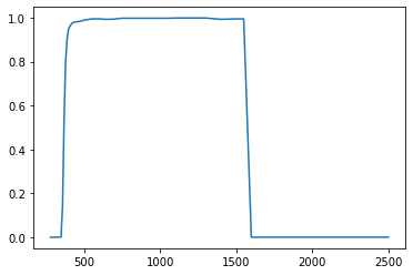
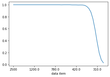
The transmission data may be plotted directly from the Series via plot()
fcd1_pd['internal transmission mm, 10'].T.plot()
<Axes: xlabel='data item'>
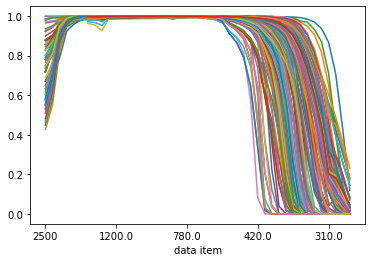
All of the glasses in the catalog DataFrame may be plotted on the same graph.
hoya_df['internal transmission mm, 10'].T.plot(legend=False)
<Axes: xlabel='data item'>
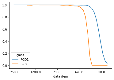
Transmission data for a list of glasses can be plotted as well.
hoya_df.loc[['FCD1', 'E-F2']]['internal transmission mm, 10'].T.plot()
<Axes: xlabel='data item'>
OpticalMedium subclasses
The glass data Series gives access to all of the vendor’s glass data, but doesn’t address the important case of using the dispersion coefficients to calculate the refractive index at an arbitrary wavelength. This is provided by catalog-specific subclasses of OpticalMedium.
fcd1 = create_glass('FCD1', 'Hoya', 'xls')
ef2 = create_glass('E-F2', 'Hoya', 'xls')
Compare measured values vs. the dispersion equation
Get the measured wavelengths. These are the indices of the 'refractive indices' category
wvls = fcd1.glass_data()['refractive indices'].index; wvls
Index([ 1529.6, 1128.64,     't',     's',    'A'',     'r',     'C',    'C'',
       'He-Ne',     'D',     'd',     'e',     'F',    'F'',     'g',     'h',
           'i'],
      dtype='object', name='data item')
The meas_rindex() method queries the refractive indices at the catalog wavelengths (the indices of the ‘refractive indices’ category).
The rindex() method uses the ‘dispersion coefficients’ to calculate the refractive index at the specified wavelength.
The following produces a table comparing the measured values to the output from the dispersion equation.
print(" wvl     meas n   interp n    delta")
for w_str in wvls:
    n_line = fcd1.meas_rindex(w_str)
    try:
        n_intrp = fcd1.rindex(w_str)
    except KeyError:
        print(f'{w_str}: {n_line}, Key error')
    else:
        print(f'{str(w_str):7s} {n_line:8.5f}  {n_intrp:8.5f}  {n_intrp-n_line:8.2g}')
 wvl     meas n   interp n    delta
1529.6   1.48598   1.48598    -4e-06
1128.64  1.48907   1.48907  -2.4e-06
t        1.49008   1.49008    -2e-07
s        1.49182   1.49182   4.9e-06
A'       1.49300   1.49300   3.3e-06
r        1.49408   1.49408  -4.9e-06
C        1.49514   1.49514  -2.5e-06
C'       1.49543   1.49543   4.1e-06
He-Ne    1.49571   1.49571   9.4e-07
D        1.49694   1.49694   2.9e-06
d        1.49700   1.49700  -2.8e-06
e        1.49845   1.49845   4.7e-07
F        1.50123   1.50123  -2.5e-06
F'       1.50157   1.50157   2.4e-06
g        1.50451   1.50451  -8.7e-07
h        1.50721   1.50721   1.2e-06
i        1.51175   1.51175  -6.4e-07
An alternative way to create an glass object
Call create_glass() on the glass catalog itself.
fcd1_v2 = hoya_xls.create_glass('FCD1')
fcd1_v2.meas_rindex('F')
np.float64(1.50123)
fcd1_v2.glass_code()
'497.816'
Plotting transmission data
The transmission_data() method returns the material transmission data for a 10mm thick sample, as well as the sample wavelengths. The data may be passed directly into matplotlib plot routines.
plt.plot(*ef2.transmission_data())
[<matplotlib.lines.Line2D at 0x175d521b0>]